Learning Generative Adversarial Networks

What is a Generative Adversial Network?

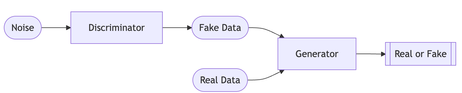
A GAN is an architecture that was motivated by the idea of creating new data. If we distill the GAN to its components, we can view it as a game. A generator takes some noise as input, and tries to transform it to some target data (with some useful distribution). At the same time, a discriminator takes a set of real data, and some fake data that has been generated via the generator, and tries to determine which are fake and which are real. In this way, the generator is effectively trying to “trick” the discriminator by creating data so convincing that the discriminator can’t accurately discern real and fake data.

Why is it useful?

GANs allow us to generate new data from noise, and therefore can be very helpful in many fields. One practical example is in medical imaging, where patient privacy might be important. Instead of using real patient information, a GAN could be trained on real patient information, and any further work could be done on fake imaging created by the generator of the trained GAN.

The Math

This section is a summary of the problem setup from the GAN paper ¹

If we let $D$ be the discriminator function, and $G$ be the generator function, consider the following scenario.

The goal is to have the generator $G$ learn some distribution $p_g$ over the dataset $\textbf{x}$. Next, consider some input noise $\textbf{z}$ with some initial distribution $p_z(\textbf{z})$. We want to have the generator map that input noise to some output that matches $p_g$, so if the generator has parameters $\theta_G$, we want to model $p_g$ from $G(\textbf{z};\theta_G)$.

At the same time, we want the discriminator $D$ to output a scalar probability that an input $\textbf{x}$ belongs to the data vs the generator’s output (which we assume becomes close to $p_g$). With parameters $\theta_D$, we can model this as $G(\textbf{x};\theta_D)$.

Since we want to train $D$ to maximize the correct label probability, while simultaenously training $G$ to minimize that the discriminators accuracy, we are playing a minimax game between the two, which can be expressed as the following functions:

Discriminator:

This function is the average accuracy of the discriminator across a single batch of real data $\textbf{x}$ and generated data from some noise $\textbf{z}$. Therefore, we need to maximize this.

Generator:

This function is the average amount of “trickery” that a generator can create when the discriminator is trying to distinguish data as real or fake.

An Example

In this example, we will try to take a $N$ dimensional uniform distribution, and use a GAN to produce a $1$ dimensional Gaussian data.

Data

The data we will use can be created easily, and this model can quickly be trained on a CPU.

Below are two functions I will be using to create the uniform noise and the real gaussian data.

def generate_gaussian(n_samples, n_dim):
    return np.random.randn(n_samples, n_dim)

def generate_uniform(n_samples, n_dim):
    return np.random.rand(n_samples, n_dim)

Models

If we transform these ideas into code, we model the generator and discriminator as basic neural networks:

class Generator(nn.Module):
    
    def __init__(self, in_feat: int, out_feat: int):
        super().__init__()
        self.fc = nn.Linear(in_feat, out_feat)
    
    def forward(self, x):
        x = F.leaky_relu(self.fc(x))
        return x

class Discriminator(nn.Module):
    
    def __init__(self, in_feat: int):
        super().__init__()
        self.fc = nn.Linear(in_feat, 1)
        
    def forward(self, x):
        x = F.sigmoid(self.fc(x))
        return x

I am using Leaky ReLU instead of ReLU to avoid gradient collapse.

Loss Functions and Instantiation

If we look at the functions in the previous section that we want to optimize, we can observe that they look similar to binary cross-entropy. In pytorch, we will use BCELoss as the loss function in both cases.

criterion = nn.BCELoss()

We also need two optimizers, one for the generator and one for the discriminator.

# data
N = 10

# models
generator = Generator(in_feat=N, out_feat=1)
discriminator = Discriminator(in_feat=1)

# optimizers
optimizer_gen = SGD(params=generator.parameters(), lr=0.01)
optimizer_disc = Adam(params=discriminator.parameters(), lr=0.01)

Training

Below is the training loop that we will use.

def train(epochs=10):
    
    BATCH_SZ = 128
    
    loss_D = []
    loss_G = []
    
    for _ in tqdm(range(epochs)):
        discriminator.zero_grad()
        
        # sample minibatch of noise and real
        noise = torch.tensor(generate_uniform(BATCH_SZ, N), dtype=torch.float32)
        real = torch.tensor(generate_gaussian(BATCH_SZ, 1), dtype=torch.float32)
        
        # get X and y
        created = generator(noise)
        x = torch.concat([real, created.detach()])
        y = torch.concat([torch.ones((BATCH_SZ,1)), torch.zeros((BATCH_SZ,1))])
        
        # update discriminator
        out1 = discriminator(x)
        loss_1 = criterion(out1, y)
        loss_1.backward()
        optimizer_disc.step()
        
        loss_D.append(loss_1.item)
        
        # update generator
        discriminator.zero_grad()
        
        out2 = discriminator(created)
        loss_2 = criterion(out2, torch.zeros((BATCH_SZ, 1)))
        loss_2.backward()
        optimizer_gen.step()
        
        loss_G.append(loss_2.item)
        
    return loss_D, loss_G

The most important part of this training loop is how we feed in the data and labels into the loss function. If we look at the loss function of BCELoss, we see the following equation:

(this is before averaging, which BCELoss does by default)

What we observe in the above equation is that $y_n$ controls the first $\log x_n$, and $1-y_n$ controls the second $\log(1-x_n)$. If we pass in some data generated from noise $G(\textbf{z})$ as $x_n$, we only want the second term, so we can set $y_n = 0$. Alternatively, if we pass in the real data, we only want to first term, so we can set $y_n=1$. Therefore, in the code above, we create the label to be $1$ for real data, and $0$ for the fake data when passed in to the loss function.

Then, when updating the generator, we only collect the loss on the fake data half, so $y_n=0$.

Evaluation

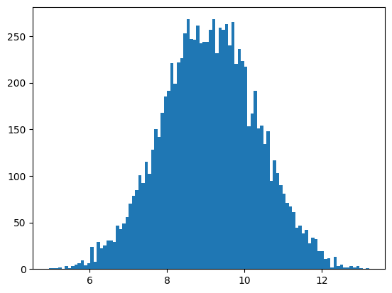
To evaluate a trained model, we can use the following code that generates some fake data from noise, and plots it. We should expect to see a Gaussian distribution in the histogram.

# evaluate
with torch.no_grad():
    noise = torch.tensor(np.random.rand(10000, N)).to(torch.float32)
    generated_samples = generator(noise).detach()

plt.hist(generated_samples, bins=100)
plt.show()

When I ran this for several hundred epochs, I achieved the following distribution:

Conclusion

GANs are powerful tools for generating data, and there are several additions to this approach that were not discussed in this post. For further reading, consider looking into DCGANs, and using GANs for other tasks like self-supervised learning and more.